Mechanical Vibration
Web Book
Forced Vibration
Learning objectives
- Derive the Frequency Response Function (FRF).
- Solve the forced vibration problems in terms of controlled mass, stiffness and damper elements.
Sections
4.1 Forcing frequency
4.2 Undamped forced vibration
4.3 Damped forced vibration
4.4 Vibration measurement

4.3 Damped forced vibration
4.3.1 Derivation of Frequency Response Function (FRF)
4.3.2 Controlled parameters and FRF plots
4.3.3 FRF in frequency ratio
4.3.4 Phase
In Section 4.2, you got the idea how dangerous the situation is, if the excitation frequency coincides with the natural frequency of a vibrating system. The vibration amplitude can (mathematically) goes into infinity.
Now the same principle can be used to derive the FRF (frequency response function) for a SDOF system with damping.
In this section, we will see the practical application of a damper in suppressing the vibration amplitude at resonance.

Figure 4.3.1 A SDOF model for a damped forced vibration.
The equation of motion for a damped SDOF system in Figure 4.3.1 is given by (watch again Video 4.2.1)
m\ddot{x}(t)+c\dot{x}(t)+kx(t)=F_e(t)=F\sin(\omega t)\phantom{xxxxx}{\color{red}(4.3.1)}
where m is the mass, c is the damping constant, k is the stiffness constant and x is the displacement with t is time, and where \dot{x}=\text{d}/\text{d}t and \ddot{x}=\text{d}^2/\text{d}t^2 .
The particular solution for the differential equation in Eq. (4.3.1) is now
x(t)=X\sin(\omega t-\theta)\phantom{xxxxxxxxxxxx}{\color{red}(4.3.2)}
where X is the magnitude of displacement and \theta is the phase shift because of the presence of damping.
In this book, the derivation of the FRF (or its magnitude) from Eq. (4.3.1) is presented using two ways: a) the vector method and b) the complex exponential notation.

4.3.1 Derivation of Frequency Response Function (FRF)
The vector method
Let us substitute Eq. (4.3.2) to each component in Eq. (4.3.1), and express each of them in the form of \sin(\omega t).
For the three force components on the left hand side of Eq.(4.3.1), namely the inertial force, the damping force and the spring force, respectively, we then have
m\ddot{x}=-\omega^2mX\sin(\omega t-\theta)\phantom{xxxxxxxxx}{\color{red}(4.3.3)}
c\dot{x}=\omega cX\cos(\omega t-\theta)=\omega cX\sin(\omega t-\theta+\tfrac{\pi}{2})\phantom{xxxxxx}{\color{red}(4.3.4)}
c\dot{x}=\omega cX\cos(\omega t-\theta)
=\omega cX\sin(\omega t-\theta+\tfrac{\pi}{2})\phantom{xxxxxxxx}{\color{red}(4.3.4)}
kx=kX\sin(\omega t-\theta)\phantom{xxxxxxxxxx}{\color{red}(4.3.5)}
Substituting Eqs. (4.3.3) to (4.3.5) to Eq. (4.3.1), we have
-\omega^2mX\sin(\omega t-\theta)+\displaystyle \omega cX\sin(\omega t-\theta+\tfrac{\pi}{2})+kX\sin(\omega t-\theta)=F\sin(\omega t)\phantom{xxxxx}{\color{red}(4.3.6)}
From Eq. (4.3.6), we can put each force in a polar plot, where the magnitude of force (in front of the sin function) is the radius, and the phase is the angle of the sin function as shown in Figure 4.3.2.

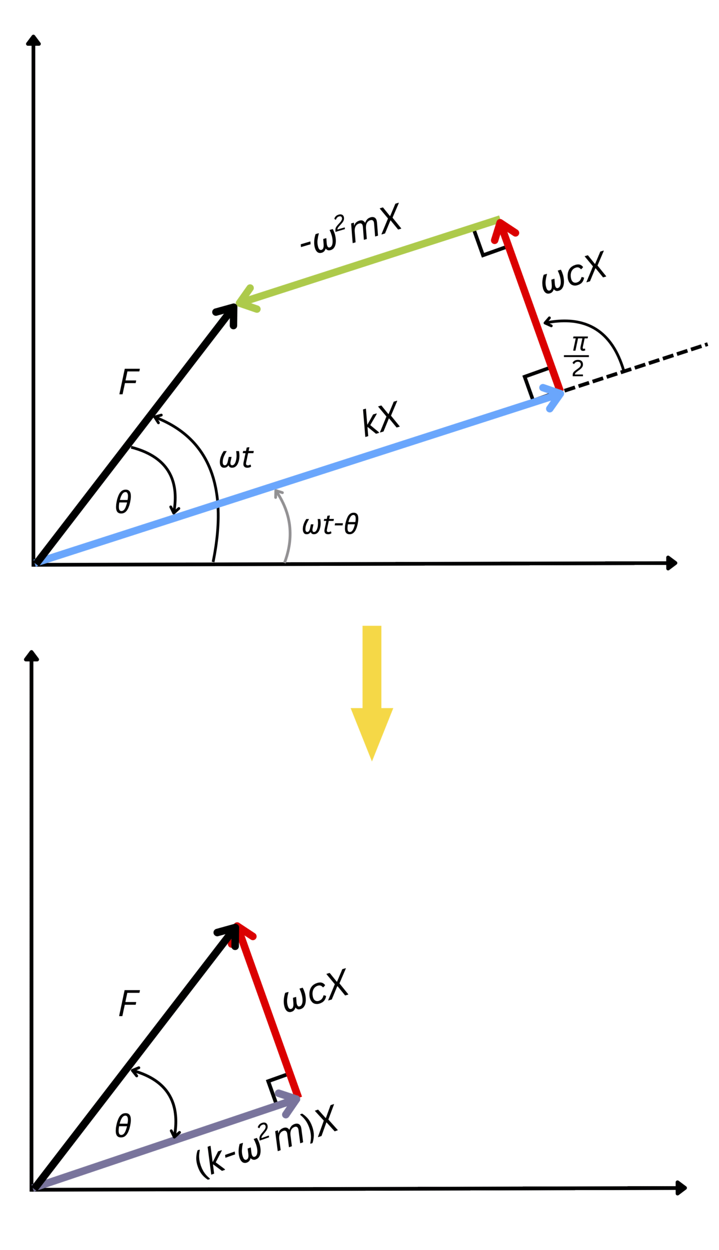
Figure 4.3.2 The vectors of forces in a SDOF, damped force vibration system.
From the vector in Figure 4.3.2, we can write
\displaystyle [(k-\omega^2m)^2+(\omega c)^2]X^2=F^2\phantom{xxxxx}{\color{red}(4.3.7)}
The magnitude of the FRF (displacement over a unit force) is therefore
\displaystyle\left|\frac{X}{F}\right|=\frac{1}{\sqrt{(k-m\omega^2)^2+(\omega c)^2}}\phantom{xxxxx}{\color{red}(4.3.8)}
The complex exponential notation
The solution of the equation of motion in Eq. (4.3.1) can also be written as
x(t)=C_1\sin(\omega t)+C_2\cos(\omega t)\phantom{xxxxxxxxxxxx}{\color{red}(4.3.9)}
where the constants C_1 and C_2 are yet to be defined.
Instead of dealing with the hard way by using Eq. (4.3.9), we can utilize the Euler’s equation which also includes the sine and cosine functions, but in complex numbers. The amplitude can be written as
x(t)=Xe^{j\omega t}=X\left[\cos(\omega t)+j\sin(\omega t)\right]\phantom{xxxxxxxxxxxxxxxx}{\color{red}(4.3.10)}
where j=\sqrt{-1} and X is now a complex number.
The Euler’s equation e^{j\theta} is denoted here as the complex exponential notation (c.e.n) .
Figure 4.3.3 shows the graphic representation of x(t)=Xe^{j\omega t} in real and imaginary coordinates. This graph also indicates that the sin function has 90-degree phase difference with the cos function ( \cos \alpha=\sin(\alpha+\tfrac{\pi}{2}) ).

Figure 4.3.3 The amplitude in complex exponential notation plotted in complex coordinates.
Since x(t)=Xe^{j\omega t} is displacement, the velocity and the acceleration can then be expressed as
v(t)=\dot{x}(t)=j\omega Xe^{j\omega t}\phantom{xxxxxxxxxx}{\color{red}(4.3.11)}
a(t)=\displaystyle\ddot{x}(t)=-\omega^2 Xe^{j\omega t}\phantom{xxxxxxxxxx}{\color{red}(4.3.12)}
By substituting x(t)=Xe^{j\omega t} into Eq. (4.3.1) and by expressing the force also in c.e.n, where F_e(t)=Fe^{j\omega t} , the term e^{j\omega t} can be canceled out and we can obtain the Frequency Response Function (FRF) of the SDOF system given by
\displaystyle\frac{X}{F}=\frac{1}{k-m\omega^2+j\omega c}\phantom{xxxxxxxxxxxx}{\color{red}(4.3.13)}
From Eq. (4.3.13), the magnitude of the FRF is
\displaystyle\left|\frac{X}{F}\right|=\frac{1}{\sqrt{(k-m\omega^2)^2+(\omega c)^2}}\phantom{xxxxx}{\color{red}(4.3.14)} )
and the phase* of the FRF is
\angle\left|\displaystyle\frac{X}{F}\right|=\phi=-\tan^{-1}\left(\displaystyle\frac{\omega c}{k-\omega^2m}\right)\phantom{xxxxxx}{\color{red}(4.3.15)}
*If z=1/(a+jb), then \angle z=\tan^{-1}(b/a)
4.3.2 Controlled parameters and FRF plots
By dividing the numerator and denominator with k in Eq. (4.3.13) and by expressing the damping constant in terms of damping loss factor \zeta, where c=2\zeta\omega_n m, we have
\displaystyle\frac{X}{F}=\frac{1/k}{1-\displaystyle\left(\frac{\omega}{\omega_n}\right)^2+j2\zeta\displaystyle\frac{\omega}{\omega}}\phantom{xxxxxxxxxx}{\color{red}(4.3.16)}
The magnitude of Eq. (4.3.16) is therefore
\left|\displaystyle\frac{X}{F}\right|=\displaystyle\frac{1/k}{\sqrt{\left[1-\displaystyle\left(\frac{\omega}{\omega_n}\right)^2\right]^2+4\zeta^2\displaystyle\frac{\omega^2}{\omega_n^2}}}\phantom{xxxx}{\color{red}(4.3.17)}
Watch Video 4.3.1 for the derivation of FRF in Eq. (4.3.16) and its magnitude in Eq. (4.3.17) using c.e.n in more details.
Video 4.3.1 Derivation of FRF of a damped forced SDOF system.
Let us now break up the magnitude |X/F| in Eq. (4.3.17) into the frequency regions relative to the natural frequency, \omega_n .
a. Stiffness controlled region
The forcing frequency is well below the natural frequency, \omega\ll \omega_n .
Because \omega/\omega_n\rightarrow 0 . the first term in the denominator will be 1-(\omega/\omega_n)^2\approx 1 .
Meanwhile the second term consists of \zeta^2 . where the damping loss factor \zeta is usually very small for a typical engineering structure, which is \zeta<0.1 . And thus 4\zeta^2(\omega/\omega_n)^2\ll 1 .
Equation (4.3.17) can then be approximated as
\displaystyle\left|\frac{X}{F}\right|\approx \frac{1}{k}\phantom{xxxxxxxxxxxxxx}{\color{red}(4.3.18)}
We can see that at low frequencies, the magnitude |X/F| is solely dependent on the stiffness constant, k (stiffness controlled). The magnitude can be reduced by increasing the stiffness.
Animation 4.3.1 FRF graph: Stiffness controlled at low frequency.
b. Damping controlled region
The forcing frequency coincides with the natural frequency, \omega= \omega_n .
From Eq. (4.3.17), as \omega/\omega_n=1 , the denominator will reduce to 2\zeta , thus
\displaystyle\left|\frac{X}{F}\right|\approx \frac{1}{2\zeta k}\phantom{xxxxxxxxxxxx}{\color{red}(4.3.19)}
This indicates that at resonance (or where the forcing frequency is in the vicinity of the resonant frequency), the magnitude |X/F| , is mainly sensitive to the change of damping, \zeta (damping controlled). The magnitude can be reduced by increasing the damping.
Animation 4.3.2 FRF graph: Damping controlled at resonance.
c. Mass controlled region
The forcing frequency is well above the natural frequency, \omega\gg \omega_n .
From Eq. (4.3.17), as (\omega/\omega_n)^2\gg 1 , the first term in the denominator becomes (\omega/\omega_n)^2\gg 1 . Thus we can write the denominator as \sqrt{(\omega/\omega_n)^4+4\zeta^2(\omega/\omega_n)^2} .
Again here, the first term is much greater than the second term, (\omega/\omega_n)^4\gg 4\zeta^2(\omega/\omega_n)^2 .
We can then simplify Eq. (4.3.17) as
\left|\displaystyle\frac{X}{F}\right|\approx \displaystyle\frac{\omega_n^2}{k\omega^2}=\frac{1}{m\omega^2}\phantom{xxxxxx}{\color{red}(4.3.20)}
At high frequencies, the magnitude |X/F| is controlled by the mass, m (mass controlled). The magnitude can be reduced by increasing the mass of the system.
Animation 4.3.3 FRF graph: Mass controlled at high frequency.
The plot of the FRF magnitude in Eq. (4.3.17) is shown in Figure 4.3.4. It must be noted that this graph is plot in logarithmic scale to better visualize the controlled regions.
Summary of FRF graph
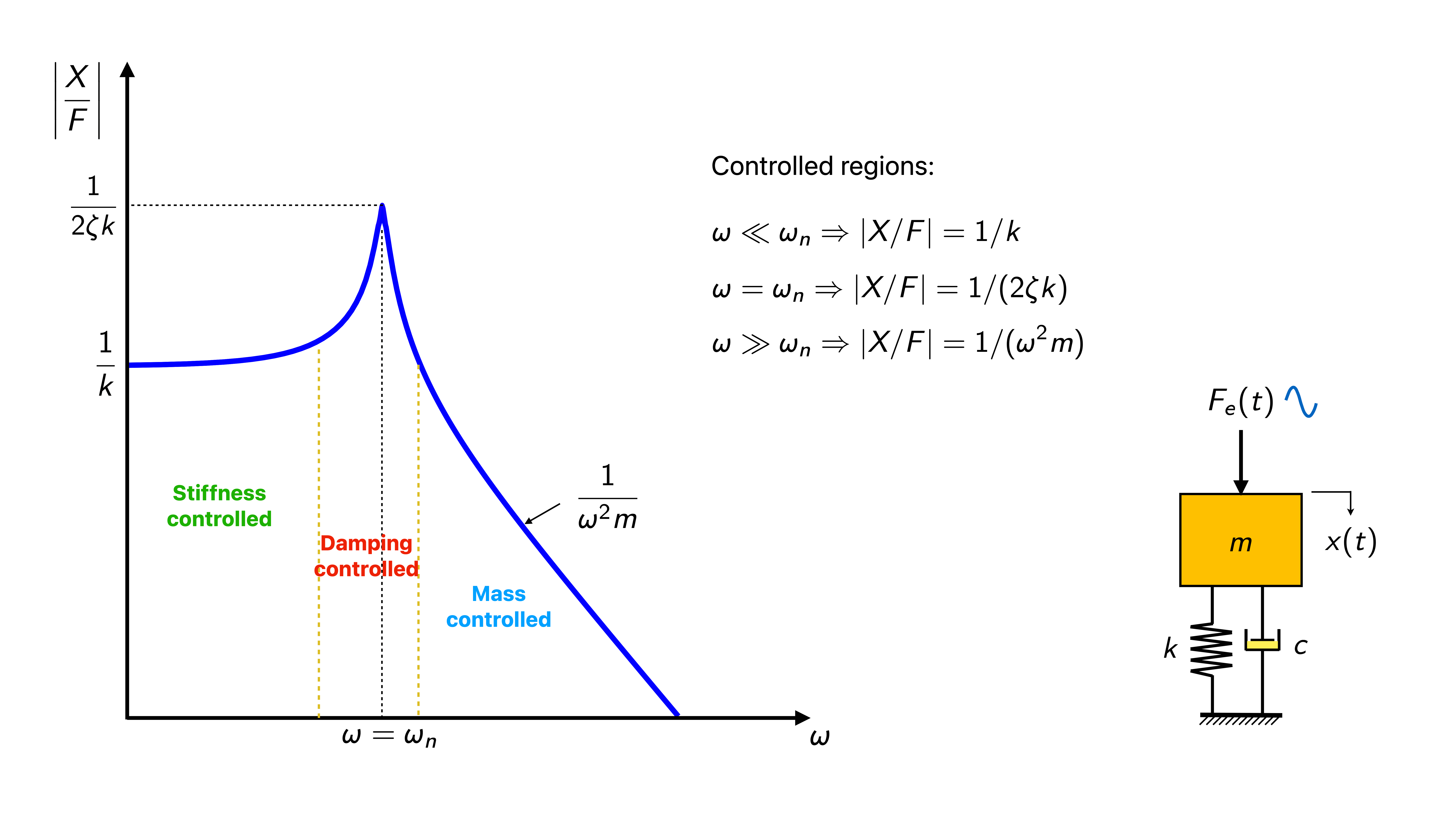
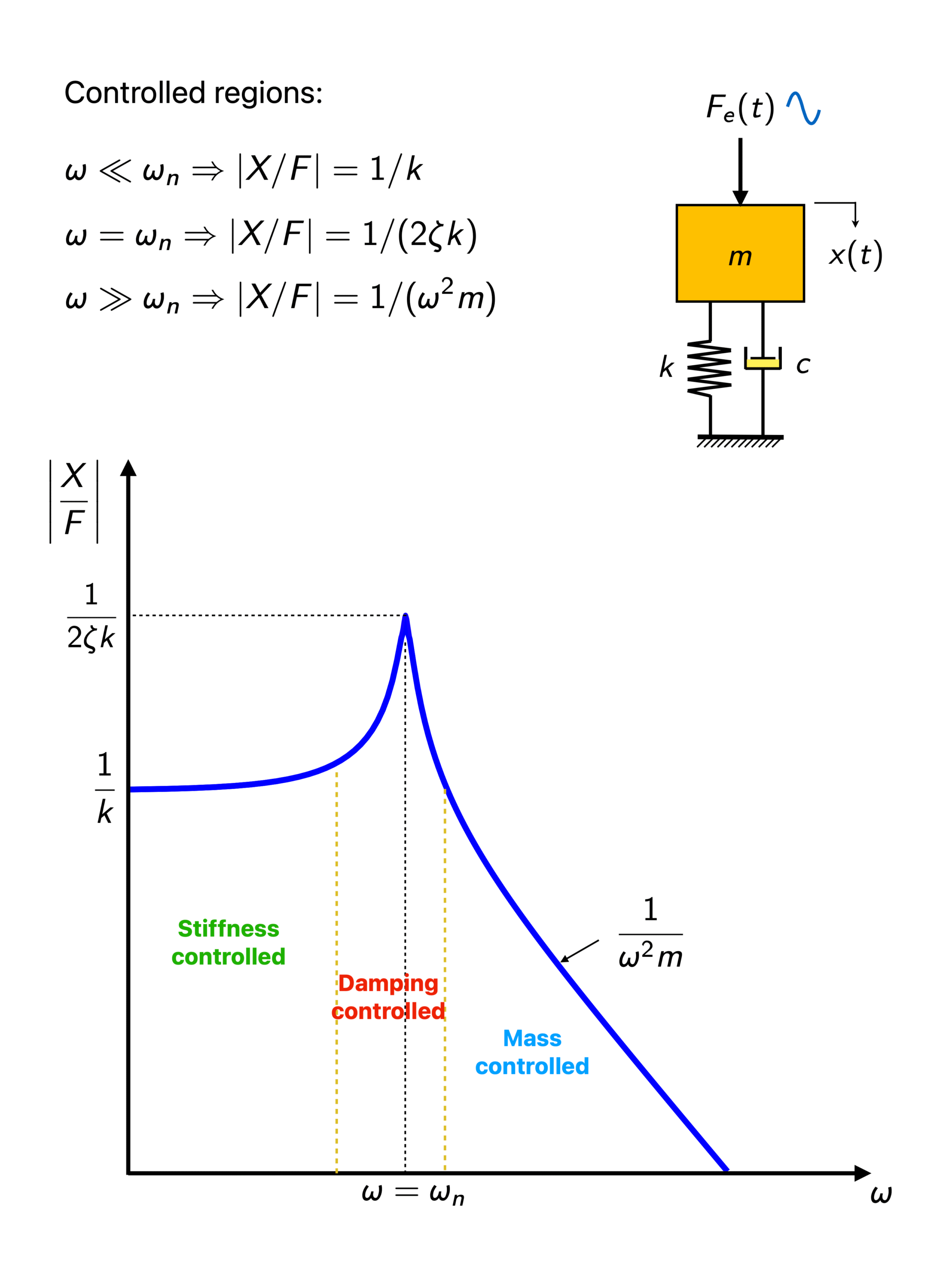
Figure 4.3.4 Plot of the FRF magnitude across the frequency and its controlled regions.
Animation 4.3.4 FRF graph with all controlled parameters.
Watch Video 4.3.2 on how the graph in Figure 4.3.4 is plotted in more details.
Video 4.3.2 Plot of FRF magnitude of a damped forced SDOF system.
Check your understanding
4.3.3 FRF in frequency ratio
The magnitude of FRF in Eq. (4.3.17) can be written in terms of the frequency ratio, i.e. between the forcing frequency and natural frequency:
r=\displaystyle\frac{\omega}{\omega_n}=\frac{f}{f_n}\phantom{xxxxxx}{\color{red}(4.3.21)}
Equation (4.3.17) can then simply be written as
\displaystyle\left|\frac{X}{F}\right|=\frac{1/k}{\sqrt{(1-r^2)^2+4\zeta^2r^2}}\phantom{xxxxxx}{\color{red}(4.3.22)}
With the “rule of thumb” (in engineering practice) where the forcing frequency must be away of 20% the natural frequency to avoid resonance, the FRF graph as the function of frequency ratio, r is shown in Figure 4.3.5.
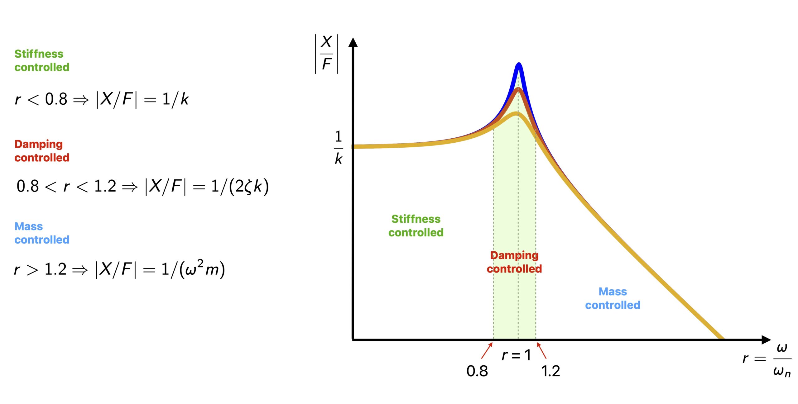
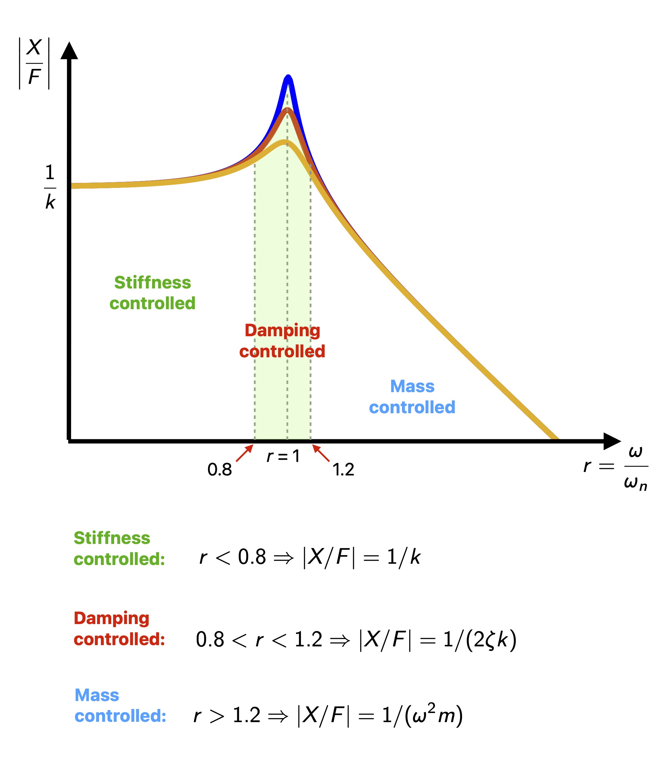
Figure 4.3.5 Plot of the FRF magnitude in the frequency ratio, r = \omega/\omega_n
The interpretation of Figure 4.3.5 is simple. If the condition is where r<0.8, then we have to increase the stiffness to reduce the vibration level. If r>1.2, then the mass must be increased.
Play with the graph in Animation 4.3.5 to make sense of Figure 4.3.5. The goal is to reduce the level of the ‘red dot’, by controlling the right parameter in the corresponding frequency region. The dashed orange lines are the area of damping controlled (0.8<r<1.2).
Animation 4.3.5 FRF graph in frequency ratio with all controlled parameters.