Mechanical Vibration
Web Book
Forced Vibration
Learning objectives
- Derive the Frequency Response Function (FRF).
- Solve the forced vibration problems in terms of controlled mass, stiffness and damper elements.
Sections
4.1 Forcing frequency
4.2 Undamped forced vibration
4.3 Damped forced vibration
4.4 Vibration measurement

4.2 Undamped forced vibration
We have derived the equation of motion for free vibration of a SDOF system as in Chapter 3. Now we have a system with an external force, F_e(t) acting on the system as shown in Figure 4.2.1.
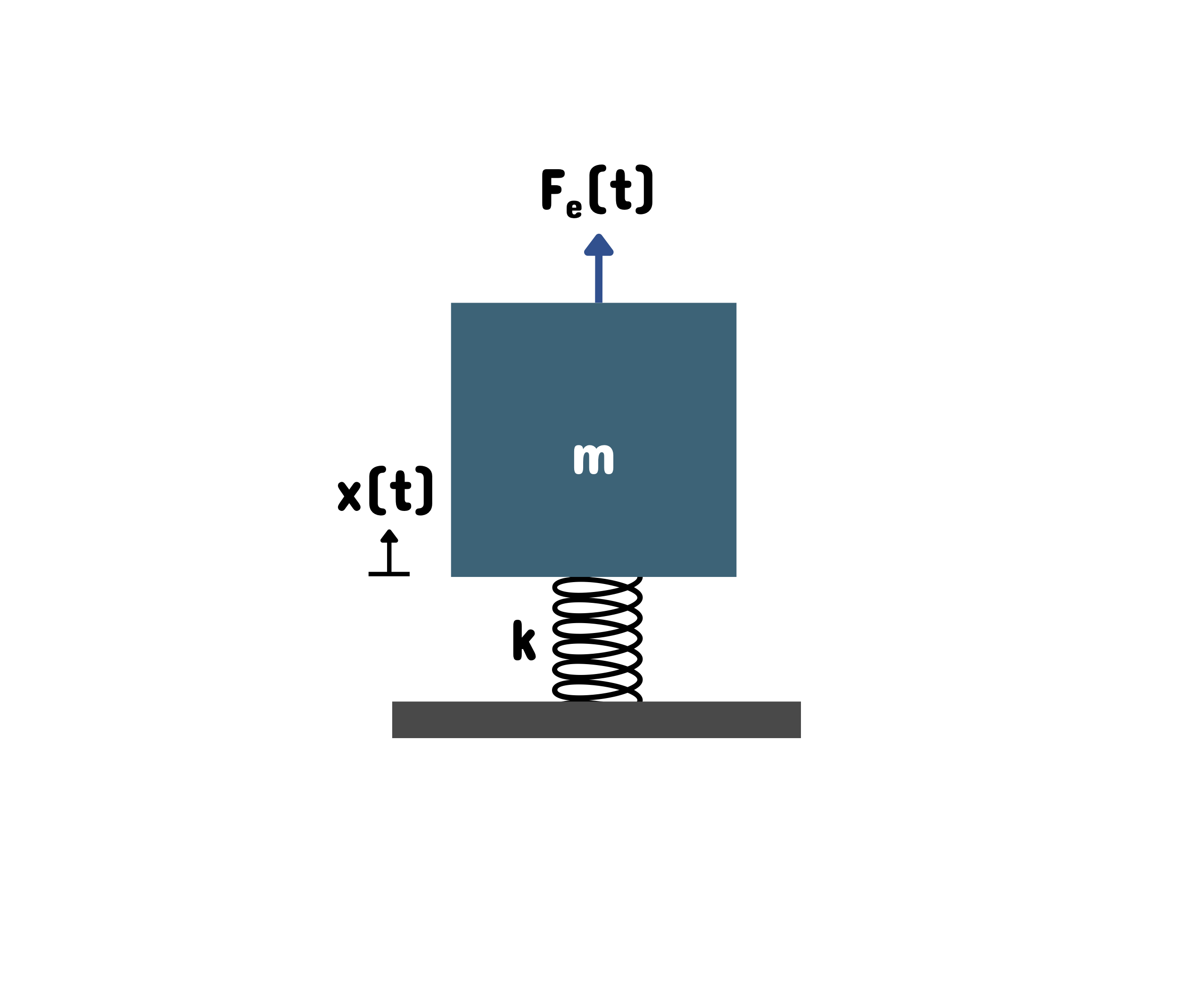
Figure 4.2.1 A SDOF model for an undamped forced vibration.
The equation of motion is given by
m\ddot{x}(t)+kx(t)=F_e(t)\phantom{xxxxxxxxxxxx}{\color{red}(4.2.1)}
where m is the mass, k is the stiffness and x is the displacement with t is time, and where \ddot{x}=\text{d}^2/\text{d}t^2 .
If the force acting on the system is a simple harmonic force (single frequency of \omega=2\pi f ) given by
F_e(t)=F\sin(\omega t)\phantom{xxxxxxxxxxxxxx}{\color{red}(4.2.2)}
where F is the magnitude of force, then the response of the system will also be harmonic expressed as
x(t)=X\sin(\omega t)\phantom{xxxxxxxxxxxxxx}{\color{red}(4.2.3)}
where X is the magnitude of displacement.
You can watch Video 4.2.1 on the derivation of the equation of motion (Eq. (4.2.1)). However this is for the damped vibration (including a damper element).
Video 4.2.1 Derivation of equation of motion for a forced vibration system.

4.2.1 How does resonance happen?
If we substitute Eqs. (4.2.2) and (4.2.3) to Eq. (4.2.1) and cancelling out \sin(\omega t), we have the relation between the displacement and force magnitudes given by
\displaystyle\frac{X}{F}=\frac{1}{k-\omega^2m}\phantom{xxxxxxxxxxxxxxxx}{\color{red}(4.2.4)}
It is convenient to analyse the problem with respect to the natural frequency of the system, \omega_n=\sqrt{k/m}.
By dividing the numerator and denominator in Eq. (4.2.4) with k, the equation can be re-rewritten as
\displaystyle\frac{X}{F}=\displaystyle\frac{1/k}{1-\displaystyle\left(\frac{\omega}{\omega_n}\right)^2}\phantom{xxxxxxxxxxxxxx}{\color{red}(4.2.5)}
Again in vibration, we are interested only in the magnitude, and so we can plot only the absolute values of Eq. (4.2.5). We can express this as
\displaystyle\left|\frac{X}{F}\right|=\frac{1/k}{\left|1-\displaystyle\left(\frac{\omega}{\omega_n}\right)^2\right|}\phantom{xxxxxxxxxxxxxx}{\color{red}(4.2.6)}
Equation (4.2.6) represents a ‘beautiful’ equation which tells us the behaviour of the system (represented by the displacement over a unit of force) as the function of the forcing frequency, \omega.
Equation (4.2.6) indicates that when the forcing frequency is closer or the same as the natural frequency, where \omega\approx\omega_n, then we have
\left|\displaystyle\frac{X}{F}\right|\approx \infty\phantom{xxxxxxxxxxxxxx}{\color{red}(4.2.7)}
This phenomenon where the forcing frequency coincides with the natural frequency and results in an exceptionally high magnitude of vibration is called resonance. The phenomenon which must be avoided in engineering.
Figure 4.2.2 plots the magnitude in Eq. (4.2.6) as the function of the forcing frequency. As the graph presents the response of the system (per unit force) across the forcing frequency, this is also known as the Frequency Response Function (FRF).
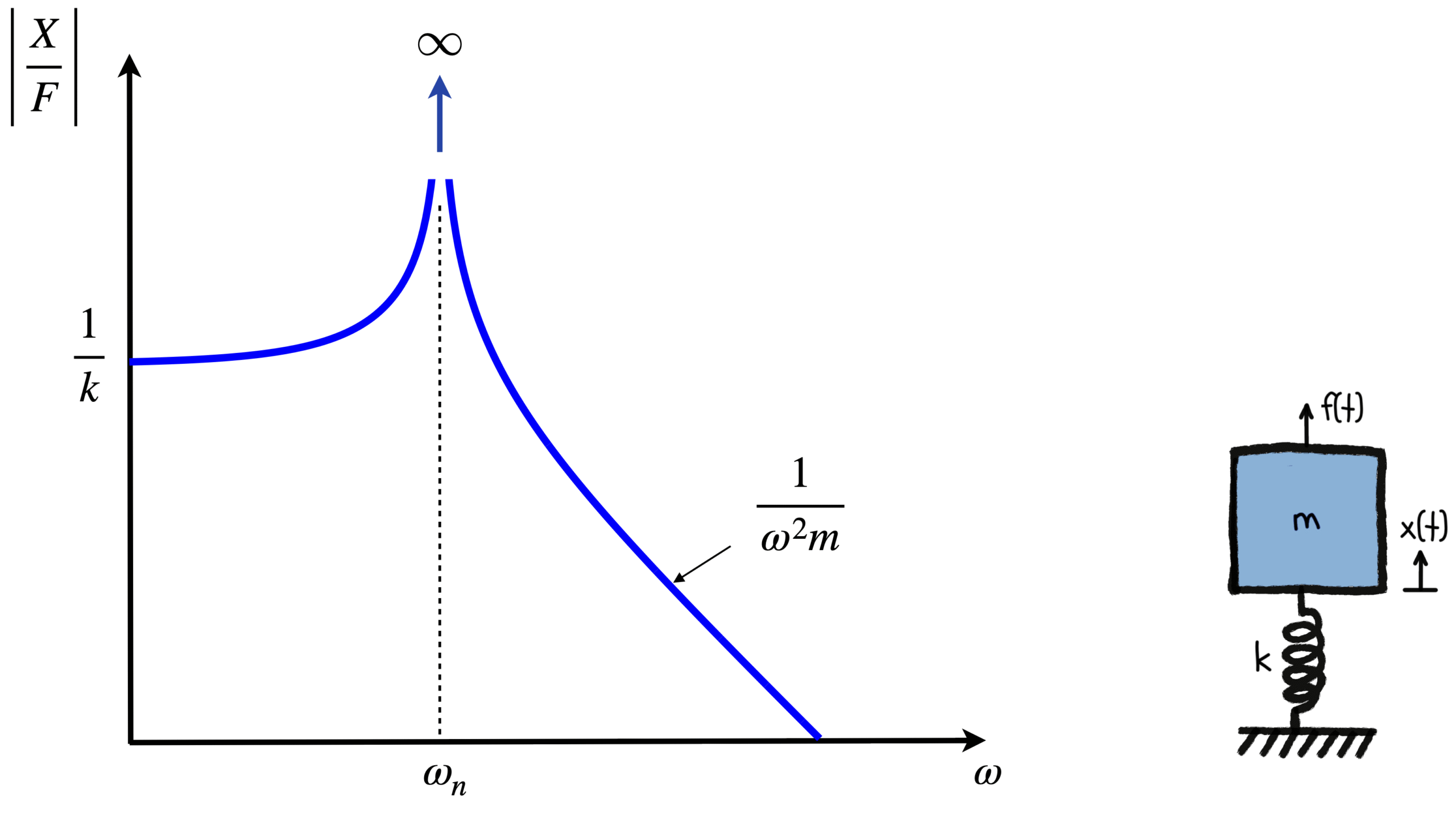
Figure 4.2.2 Plot of FRF of an undamped SDOF system.
Animation 4.2.1 shows that as the forcing frequency approaches and aligns with the natural frequency, the vibration amplitude increases dramatically.
Animation 4.2.1 Vibration response per 1 N for an undamped SDOF system.
In Video 4.2.2, you can watch how the FRF is derived until the graph is plotted from the equation.
Video 4.2.2 Derivation of FRF of an undamped SDOF system.
4.2.2 What is the impact of resonance?
The real vibration magnitude that we feel is in the time domain (time waveform). But how is the vibration magnitude in time domain at the resonance? Does it still follow the sin or cos functions?
At resonance, the assumption of harmonic response as in Eq. (4.2.3) is no longer valid. From Inman (2011), the particular solution for the vibration response must be given by
x(t)=tX\sin(\omega t)\phantom{xxxxxxxxxxxxxx}{\color{red}(4.2.8)}
Substituting to Eq. (4.2.1) and solve for X yields X\approx F/(2\omega) and thus Eq. (4.2.8) can be expressed as
x(t)=\displaystyle\frac{F}{2\omega}t\sin(\omega t)\phantom{xxxxxxxxxxxxxx}{\color{red}(4.2.9)}
Animation 4.2.2 plots the response for \omega=\omega_n=\sqrt{k/m} from condition at rest (x(0)=0) and (v(0)=0)).
The amplitude can be seen to grow as the time increases with slope of Ft/2\omega. If we have a more flexible system, i.e. with lower stiffness k, the slope will be larger, which means the time to reach the failure condition is faster.
Animation 4.2.2 Amplitude of vibration in time domain at resonant frequency
.
The phenomenon of resonance leading to structural failure happened to the Tacoma Bridge, USA in 1940 (as seen in Video 4.2.3). It was the 3rd longest suspension bridge that spanned a strait. The excitation force came from the wind (aerodynamic force) which generated vortex shedding flow and caused twisting motion which gradually increased in amplitude.
Video 4.2.3 The structural failure of Tacoma Bridge due to vibration in 1940.
Resonance is when the forcing frequency coincides with the natural frequency of a structure.