Mechanical Vibration
Web Book
Vibration Isolation
Learning objectives
- Derive the Frequency Response Function (FRF).
- Solve the forced vibration problems in terms of controlled mass, stiffness and damper elements.
Sections
5.1 Force transmissibility
5.2 Base excitation
5.3 Vibration measurement

5.1 Force Transmissibility

5.1.1 Introduction
Figure 5.1.1 shows a rotating machine (source) installed rigidly on a floor, where the injected vibration energy is propagating through the floor (path) and vibrates the office table (receiver).
In this scenario, the sensitive location that requires vibration control is the table. While the source may have an acceptable vibration level, the transmitted vibration to the receiver can be disruptive or hazardous in various situations.
Figure 5.1.1 Illustration of vibration transmission from the source to the receiver.
Practically, to reduce the vibration, we can do the followings:
- Reduce vibration at the source. This is the ideal way, but mostly cannot be done as the machine is naturally rotating and has the potential to inject a dynamic force. The force will be greater if machine has balancing problem.
- Modify the transmission path. This is what will be discussed in this chapter. The idea is to block some of the vibration energy going to the receiver at the connection between the source and the receiver.
- Control at receiver. Add damping to the table. This will be costly if excessive damping is required.
5.1.2 What is Transmissibility?
Let us focus on the machine in Figure 5.1.1, where it is assumed to have excitation force with magnitude F and it transmits vibration force to the floor with magnitude F_T .
We can express the ratio of these two forces as
T=\displaystyle\left|\frac{F_t}{F}\right|\phantom{xxxxxxxxxxxxxx}{\color{red}(5.1.1)}
which is termed as transmissibility.
For the vibration control measure, the goal is to have the transmitted force, F_T as small as possible compared to the excitation force, F . This indicates that we have ‘blocked’ some of the vibration energy that goes into the receiver structure.
Our goal must be
T<1\phantom{xxxxxxxxxxxxxx}{\color{red}(5.1.2)}
which means the closer T to the zero value, the better.
From Figure 5.1.2, the only path the vibration energy can get into the floor, is through the mounting of the machine. And this is what we will design to reduce the transmitted force F_T .
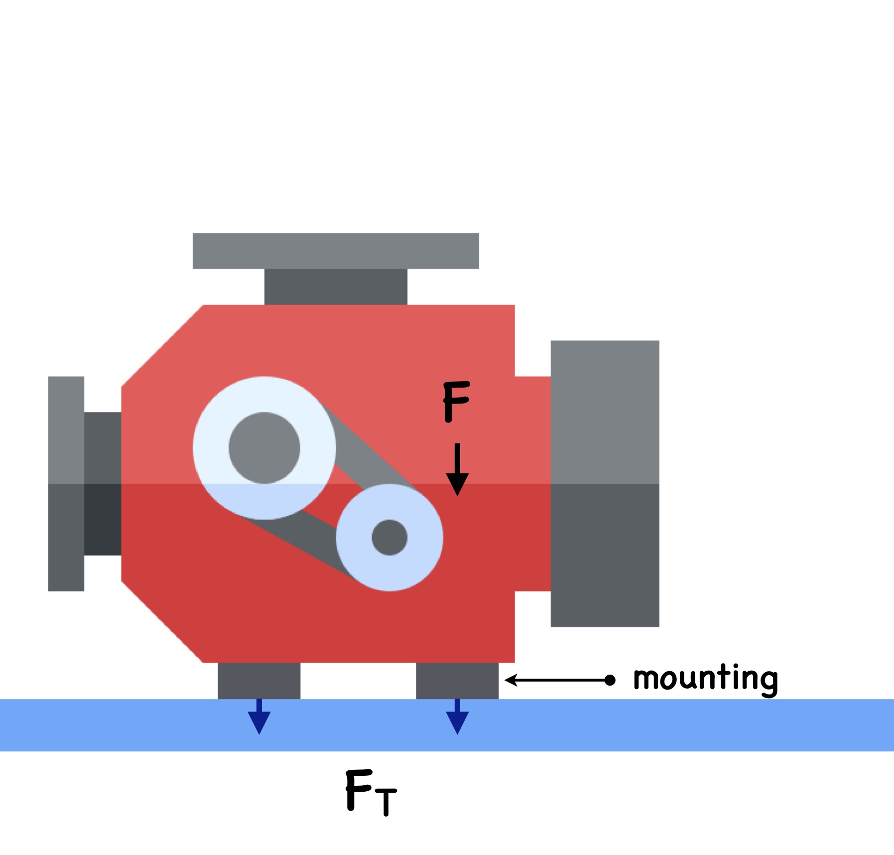
Figure 5.1.2 Excitation force and transmitted force through mountings.
Let’s go into the math!
5.1.3 Derivation of Transmissibility equation
In Figure 5.1.3, the machine system is assumed to have a rigid mass, m oscillating on flexible mountings with stiffness constant, k and damping constant, c
The machine excites harmonic force, F(t) and to have the transmitted force, F(t) on the floor, where the floor is modeled as a rigid base (we obtain the blocked force). The single-degree-of-freedom system can then be constructed with the mass having amplitude of vibration, x(t) .
Figure 5.1.3 Single-degree-of-freedom (SDOF) model for force transmissibility.
The floor directly receives the injected force only from two components, i.e. from the spring and the damper. Thus the transmitted force is a total force from the damping and spring forces expressed as
f_T(t)=c\dot{x}(t)+kx(t)\phantom{xxxxxxxxxxxx}{\color{red}(5.1.3)}
Meanwhile the excitation force includes the inertial force from the mass written as
f(t)=m\ddot{x}(t)+c\dot{x}(t)+kx(t)\phantom{xxxxxx}{\color{red}(5.1.4)}
For ease of deriving the equation, we use the complex exponential notation (revisit again here) to represent the harmonic function, so that
f_T(t)=F_Te^{j\omega t}\phantom{xxxxxxxxxxxx}{\color{red}(5.1.5)}
and
f(t)=Fe^{j\omega t}\phantom{xxxxxxxxxxxx}{\color{red}(5.1.6)}
where F_T and F are complex amplitudes, \omega is the forcing frequency (in rad/s), and where j=\sqrt{-1} .
The solution for Eqs. (5.1.3) and (5.1.4) is also in the form of complex exponential notation given as
x(t)=Xe^{j\omega t}\phantom{xxxxxxxxxxxx}{\color{red}(5.1.7)}
By substituting Eqs. (5.1.5)-(5.1.7) to Eqs. (5.1.3) and (5.1.4), the ratio of the transmitted force to the excitation force is given by
\displaystyle \frac{F_T}{F}=\displaystyle \frac{k+j\omega c}{k-\omega^2m+j\omega c}\phantom{xxxxxxxxxxxxxx}{\color{red}(5.1.8)}
Note that the terms e^{j\omega t} and Xe^{j\omega t} have been cancelled out in Eq. (5.1.8).
By first dividing both the numerator and denominator on the right-hand side of Eq. (5.1.8) by stiffness constant k and by defining the damping constant as c=2\zeta\omega_n m and \omega_n^2=k/m we obtain
\displaystyle\frac{F_T}{F}=\displaystyle\frac{1+j2\zeta\displaystyle\frac{\omega}{\omega_n}}{1-\displaystyle\left(\frac{\omega}{\omega_n}\right)^2+j2\zeta\displaystyle\frac{\omega}{\omega_n}}\phantom{xxxxxxxxxxx}{\color{red}(5.1.9)}
Equation (5.1.9) is still in complex number. The transmissibility as defined in Eq. (5.1.1) is then the modulus of Eq. (5.1.9) expressed as ^{\dagger}
T=\displaystyle\left|\frac{F_T}{F}\right|=\displaystyle\sqrt{\frac{1+4\zeta^2\displaystyle\frac{\omega^2}{\omega_n^2}}{\left[1-\displaystyle\left(\frac{\omega}{\omega_n}\right)^2\right]^2+4\zeta^2\displaystyle\frac{\omega^2}{\omega_n^2}}}\phantom{xxxxx}{\color{red}(5.1.10)}
^{\dagger} Modulus of a complex number: z=\displaystyle\frac{a+jb}{c+jd} \rightarrow |z|=\displaystyle\sqrt{\frac{a^2+b^2}{c^2+d^2}}
Watch Video 5.1.1 for the ‘visual’ derivation of Transmissibility in Eq. (5.1.10).
Video 5.1.1 Derivation of Transmissibility equation.
5.1.4 Plotting the Transmissibility graph
To understand what Eq. (5.1.10) implies in physics, let us plot the graph of transmissibility as the function of the frequency \omega . We can breach the frequency into three regions as what we have done in previous chapter.
a. The forcing frequency is much lower than the natural frequency: \omega\ll \omega_n
Because \omega/\omega_n\ll 1 , the numerator in Eq. (5.1.10) will have 4\zeta^2\omega^2/\omega_n^2\ll 1 , then 1+4\zeta^2\omega^2/\omega_n^2 \approx 1 . The same way in the denominator, it will only be left by 1. Thus
T=\displaystyle\left|\frac{F_T}{F}\right|\approx 1 \phantom{xxxxx}{\color{red}(5.1.11)}
which means at low frequency (below the natural frequency of the system), the force is transmitted effectively to the receiver structure with the same level of magnitude with that of the excitation force, |F_T|=|F |. There is no discernible impact of vibration isolation at this low frequency.
b. The forcing frequency is the same as the natural frequency: \omega=\omega_n
Equation (5.1.10) then becomes
T=\displaystyle\left|\frac{F_t}{F}\right|\approx \sqrt{\frac{1+4\zeta^2}{4\zeta^2}}\phantom{xxxxxxxxx}{\color{red}(5.1.12)}
As the damping loss factor is usually small value, where 0.01 <\zeta < 0.2, then the numerator becomes 1+4\zeta^2\approx 1 . So that
T=\displaystyle\left|\frac{F_t}{F}\right|\approx \sqrt{\frac{1}{4\zeta^2}}=\frac{1}{2\zeta}\phantom{xxxxxxx}{\color{red}(5.1.13)}
With the value of 1/(2\zeta) will always be greater than 1, this means that at resonance, the transmissibility is amplified, where the transmitted force can be significantly greater than the excitation force |F_T|>|F| .
For example if \zeta=0.1 , then |F_T|=5\times|F| .
The force transmitted into the receiver structure is five times the excitation force. This dangerous phenomenon must be avoided.
c. The forcing frequency is well above the natural frequency: \omega\gg\omega_n
If \omega\gg\omega_n , then in the numerator in Eq. (5.1.10) we have 4\zeta^2\omega^2/\omega_n^2\gg 1 , and so it is left with only 4\zeta^2\omega^2/\omega_n^2 . In the denominator, the first term in the bracket becomes [1-(\omega/\omega_n)^2]^2\approx [-(\omega/\omega_n)^2]^2=(\omega/\omega_n)^4 , which is much greater to the second term 4\zeta^2\omega^2/\omega_n^2 .
So Eq. (5.1.10) can be simplified to
T=\displaystyle\left|\frac{F_t}{F}\right|=\displaystyle\sqrt{\frac{4\zeta^2\displaystyle\frac{\omega^2}{\omega_n^2}}{\displaystyle\left(\frac{\omega}{\omega_n}\right)^4}}=\displaystyle\frac{2\zeta\omega_n}{\omega}\phantom{xxxxx}{\color{red}(5.1.14)}
Figure 5.1.4 presents the Transmissibility graph. It highlights the intended isolation area where T< 1. Conversely, the amplification area is also indicated where T> 1, which should be avoided.
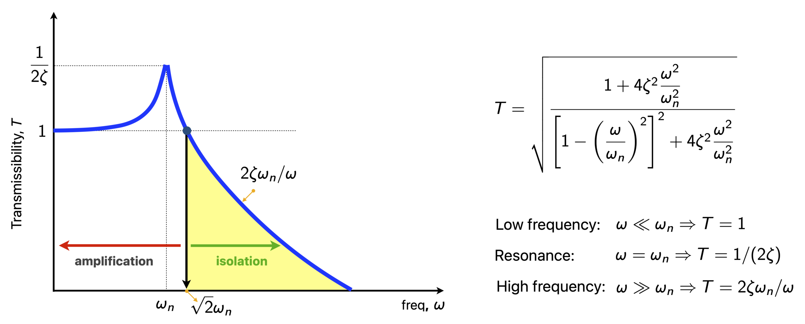
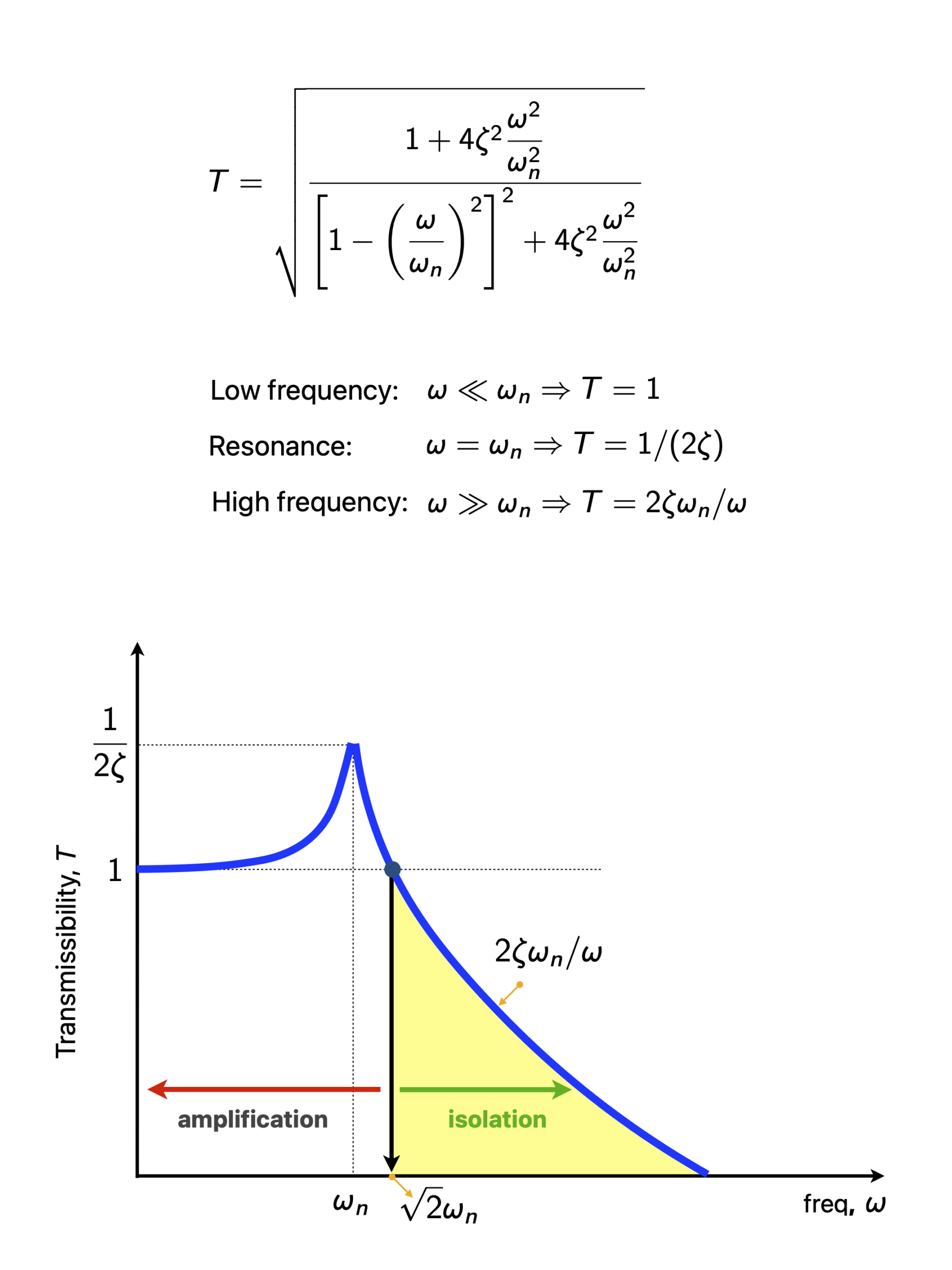
Figure 5.1.4 Transmissibility as a function of forcing frequency.
Watch Video 5.1.2 to see how the graph is plotted from Eq. (5.1.10). In this video, the transition frequency \omega=\sqrt{2}\omega_n is also derived.
Video 5.1.2 Plotting the graph of Transmissibility.
5.1.5 Transition frequency and resilient mounts
Equation (5.1.10) will look a bit simpler if we express it in terms of the frequency ratio, r=\omega/\omega_n.
T=\displaystyle\left|\frac{F_T}{F}\right|=\displaystyle\sqrt{\frac{1+4\zeta^2r^2}{\left[1-r^2\right]^2+4\zeta^2r^2}}\phantom{xxxxxxxxxx}{\color{red}(5.1.15)}
From Figure 5.1.4, the transition frequency to the isolation region can be observed to start just before T rolling off to less than unity.
Assuming small damping (\zeta\approx 0), from Eq. (5.1.15) we have
T=\displaystyle\sqrt{\frac{1}{\left[1-r^2\right]^2}}<1\phantom{xxxxxxxxxx}{\color{red}(5.1.16)}
Prior to commencing the solution, please note the denominator of Eq. (5.1.16). As depicted in Figure 5.1.4, within the isolation region, the ratio r=\omega/\omega_n will always be greater than unity, \omega/\omega_n>1. So the term [1-r^2] in Eq. (5.1.16) will always be negative.
However, as this term is squared, that is [1-r^2]^2, whatever value inside the square bracket becomes positive. And this is always true as the Transmissibility is always positive.
Thus when we eliminate the power of two with the square root in Eq. (5.1.16), the term in the square bracket in the denominator must be changed in position to maintain T to be always positive. We write
T=\displaystyle \frac{1}{r^2-1}<1\phantom{xxxxxxxxxx}{\color{red}(5.1.17)}
By re-arranging Eq. (5.1.17) to solve for r, we obtain the transition frequency of the isolation region given by
r>\sqrt{2}\phantom{xxxxxxxxxx}{\color{red}(5.1.18)}
Equation (5.18) indicates that the forcing frequency must be above \sqrt{2}\omega_n for T to be less than unity (isolation), that is
\omega>\sqrt{2}\omega_n\phantom{xxxxxxxxxx}{\color{red}(5.1.19)}
In practice, what the engineer does is not controlling the forcing frequency (operating frequency) of the machine, but to adjust the structural parameters, \omega_n.
We can re-write Eq. (5.1.19) to be
\omega_n<\displaystyle\frac{\omega}{\sqrt{2}}\phantom{xxxxxxxxxx}{\color{red}(5.1.19)}
where \omega_n=\sqrt{k/m}, with k the stiffness of the mounting, and m mass of the machine.
Equation (5.1.19) states that if we know the forcing frequency, then we should choose a resilient mounting (low k ) so that Eq. (5.1.19) can be satisfied (to be in the isolation region). This type of mounting is well-known as vibration isolators.
Figure 5.1.5 summarises on why we need resilient mountings for vibration isolation.
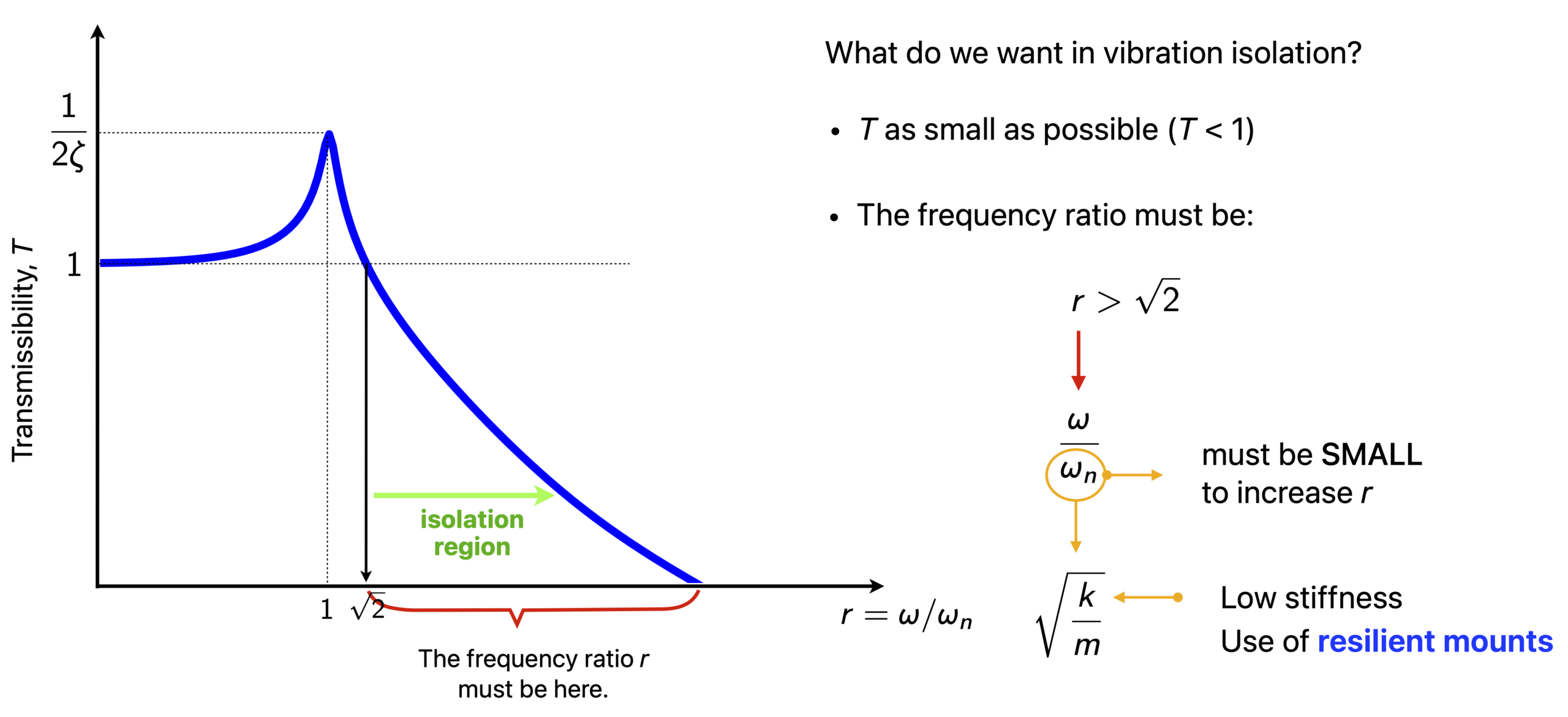
Figure 5.1.5 Summary of transition frequency and why resilient mounts?
In Animation 5.1.1 below, change k, m and \zeta to place the forcing frequency, \omega_o in the isolation region.
Animation 5.1.1 Adjusting the structural parameters to achieve vibration isolation. Which parameter is the most sensitive?
If the frequency is in frequency ratio r as in Animation 5.1.2, the objective is to shift r_o to the isolation region.
Animation 5.1.2 Adjusting the structural parameters to shift r into the vibration isolation area.
Figure 5.16 shows the application of vibration isolators and Figure 6.17 is types of isolators.
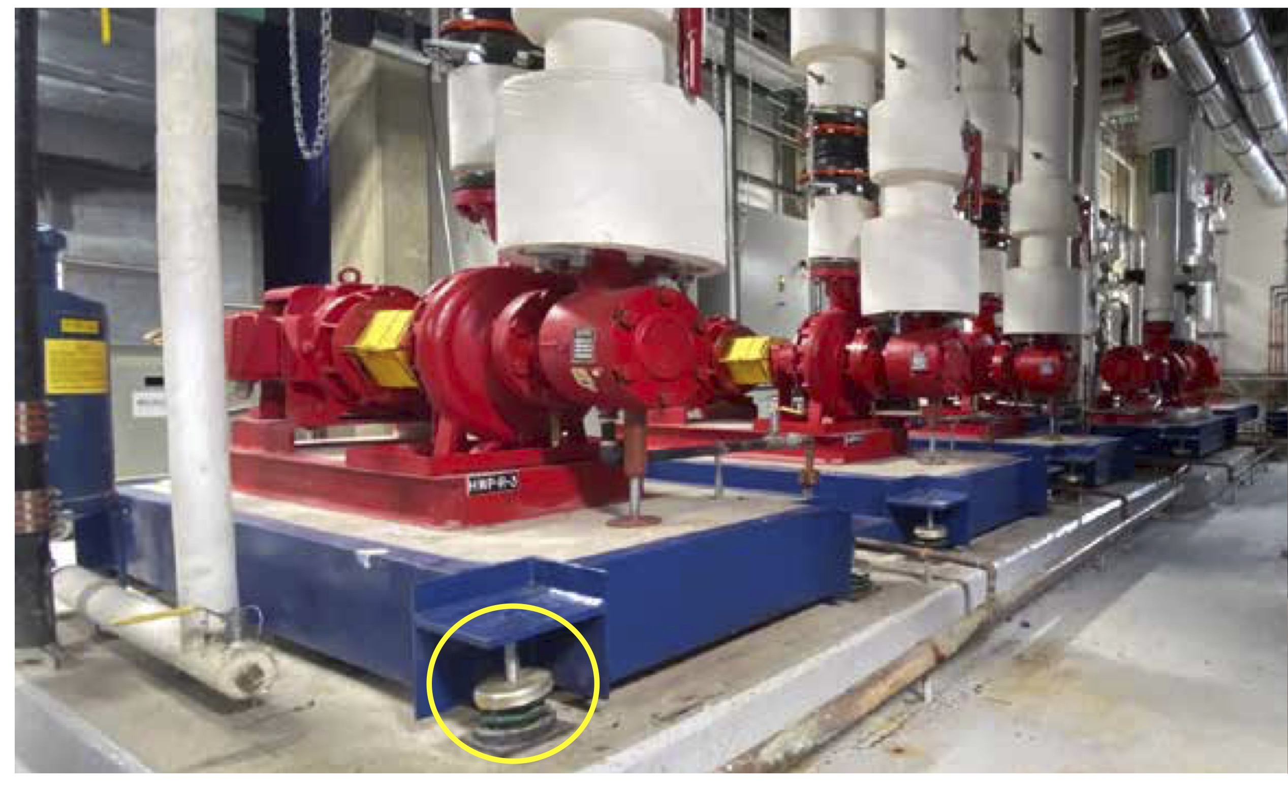
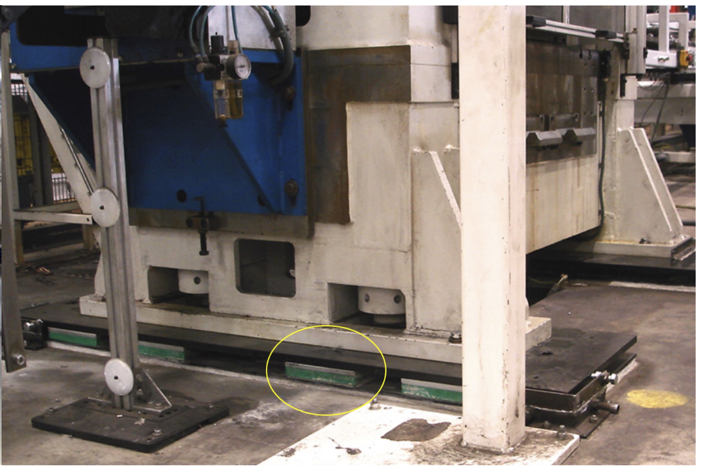
Figure 5.1.6 Application of vibration isolators to reduce vibration transmission to the base structure (Images courtesy of Kinetics Noise Control, Inc).
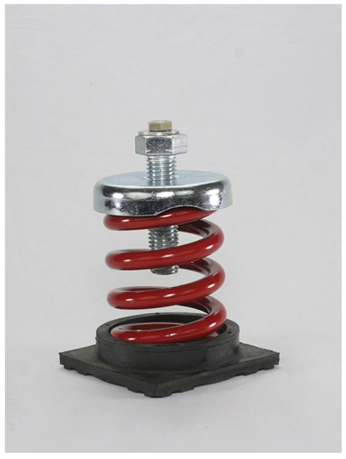
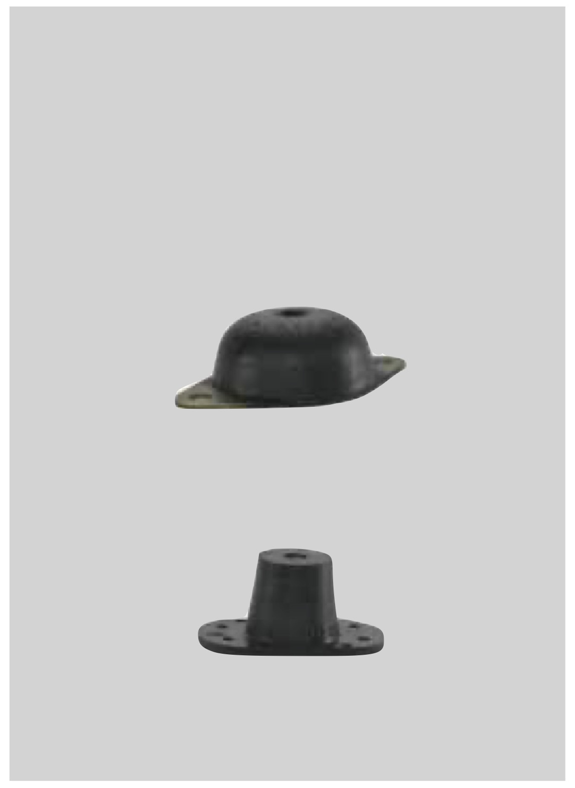
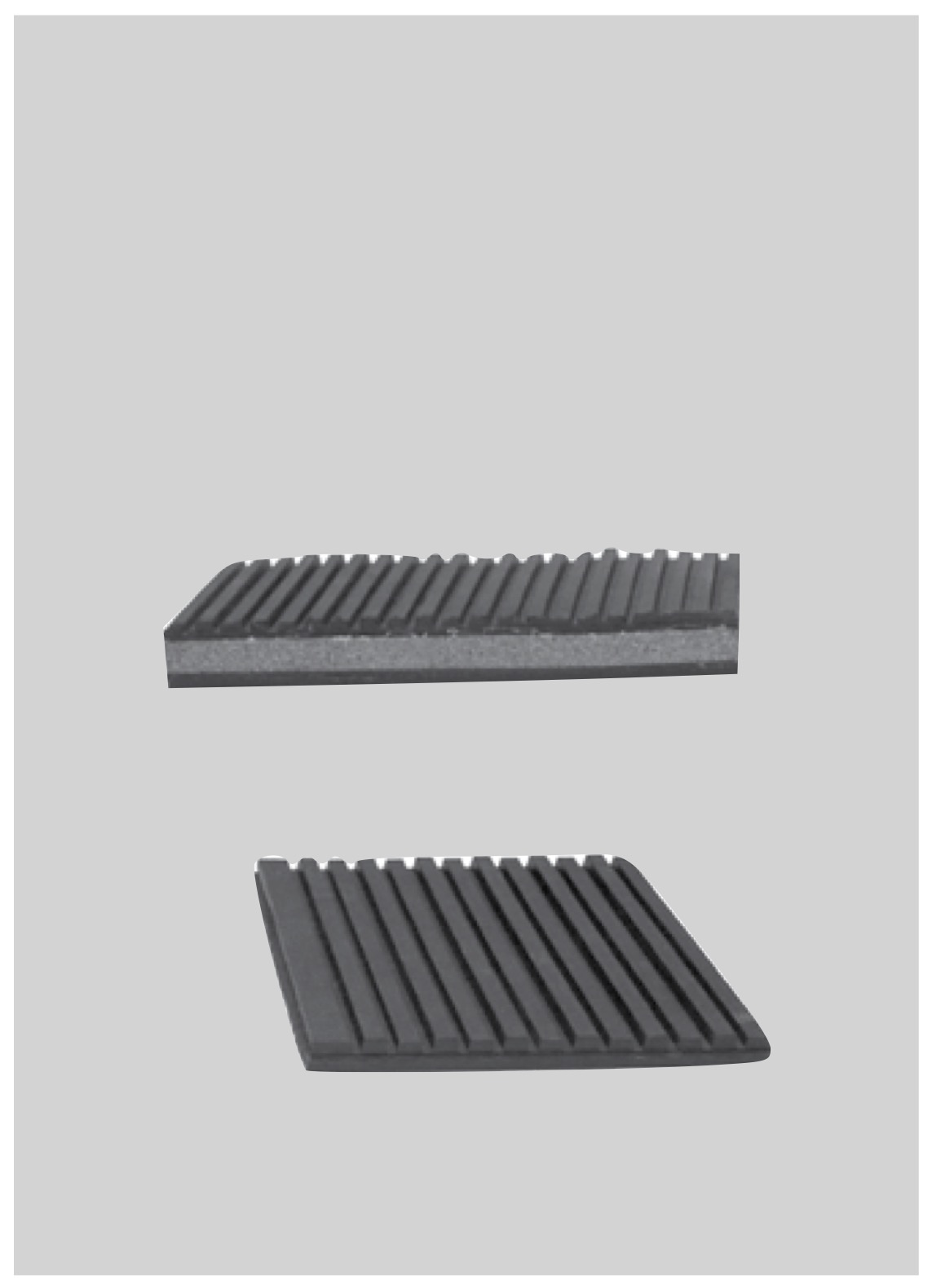
Figure 5.1.7 Spring floor isolator (for low speed machine: reciprocating compressor, centrifugal fan) [LEFT], Neoprene isolation mounts (small pump, vent set) [MIDDLE], (c) Neoprene isolation pads (for high frequency isolation, machines located on a grade-supported structural slab) [RIGHT]
(Photo courtesy of Kinetics Noise Control, Inc).
Figure 5.1.7 Spring floor isolator (for low speed machine: reciprocating compressor, centrifugal fan) [TOP], Neoprene isolation mounts (small pump, vent set) [MIDDLE], (c) Neoprene isolation pads (for high frequency isolation, machines located on a grade-supported structural slab) [BOTTOM]
(Photo courtesy of Kinetics Noise Control, Inc).
5.1.6 Effect of damping
From Eq. (5.1.14), we can see that Transmissibility is proportional to damping ratio, \zeta. This indicates that the greater the damping, the greater the Transmissibility.
Figure 5.1.5 illustrates the relationship between Transmissibility and damping ratios. It is evident that damping can substantially reduce the amplitude at resonance, which is advantageous during the machine’s startup (ramp-up) phase when the speed must surpass the natural frequency before attaining the normal operating speed.
However as seen in the graph, at the isolation region, the damping takes into effect on increasing the Transmissibility (reduction of isolation performance) at damping ratio \zeta=0.2 or larger.
When \zeta<0.2, for most isolators without special treatment of damping, the effect of damping is negligible.
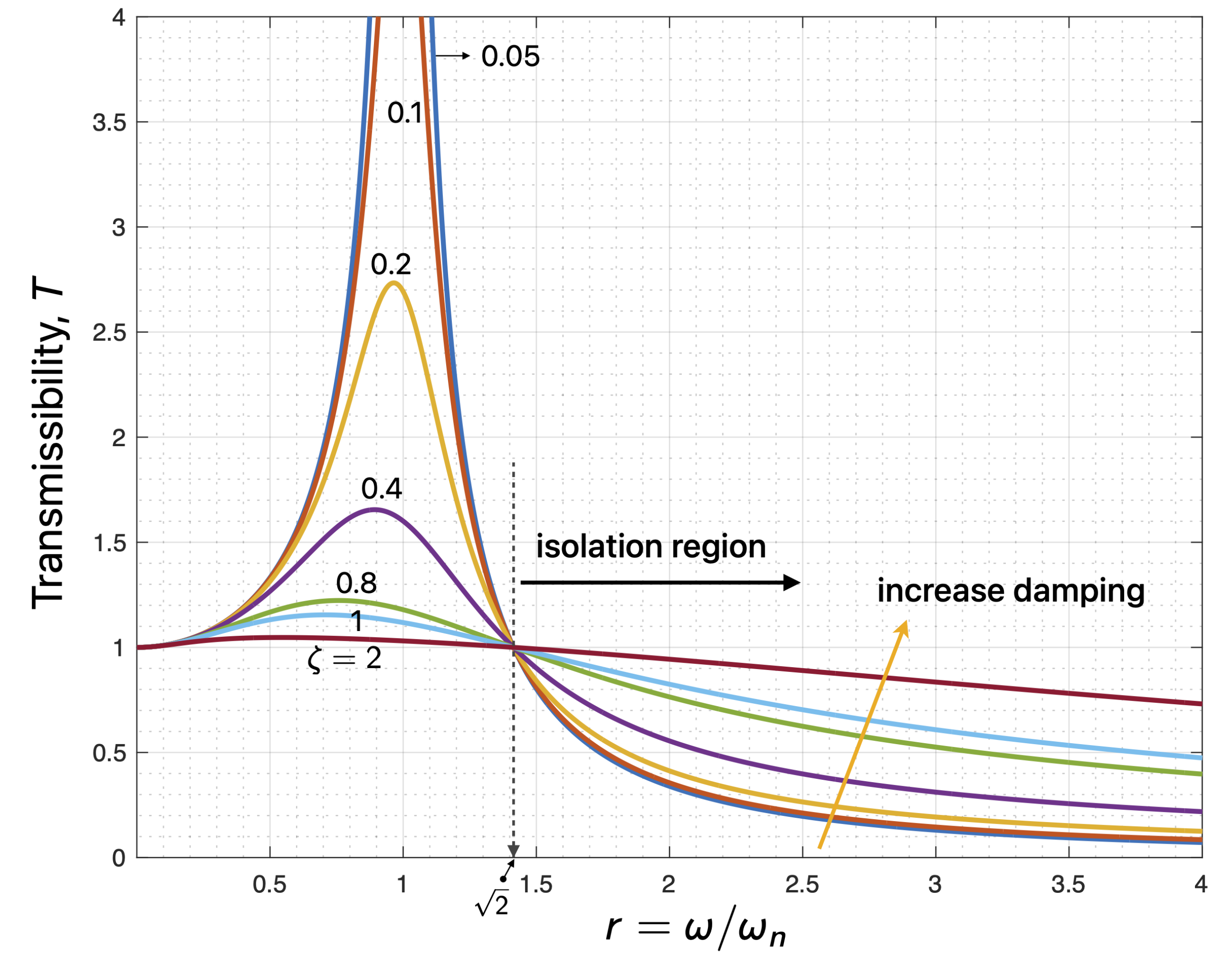
Figure 5.1.5 Transmissibility with different damping ratios.
Play with the graph in Animation 5.1.3. Change the damping ratio \zeta, and observe how T is significantly reduce around the resonant frequency (r=1).
Additionally, observe that transmissibility within the isolation region begins to increase when \zeta exceeds 0.15.
Animation 5.1.3 Effect of damping in Transmissibility.
Control at resonance
Increasing damping means reducing the performance at the isolation area.
Conversely, damping is necessary to prevent excessive vibration amplitude in the event of resonance.
For example a high speed machine during ramp-up or coast down will pass through its ‘critical frequency’ (natural frequency). The solution is to add more damping to suppress the vibration amplitude when the machine speed coincided with the natural frequency.
Animation 5.1.2 Illustration of ramp-up mode in a rotating machine.
Watch Video 5.1.3 to see how we can relate the structural parameters with the T-curve.
Video 5.1.3 Parametric analysis on the T-curve.
5.1.7 Isolation Reduction and Static Deflection
Isolation reduction
To quantify the success of isolation, it is more convenient to say:
“How many percent of vibration reduction can be achieved?”
The level of reduction is simply given by
R=(1-T)\times 100\%\phantom{xxxxxxxxx}{\color{red}(5.1.16)}
where T is the Transmissibility.
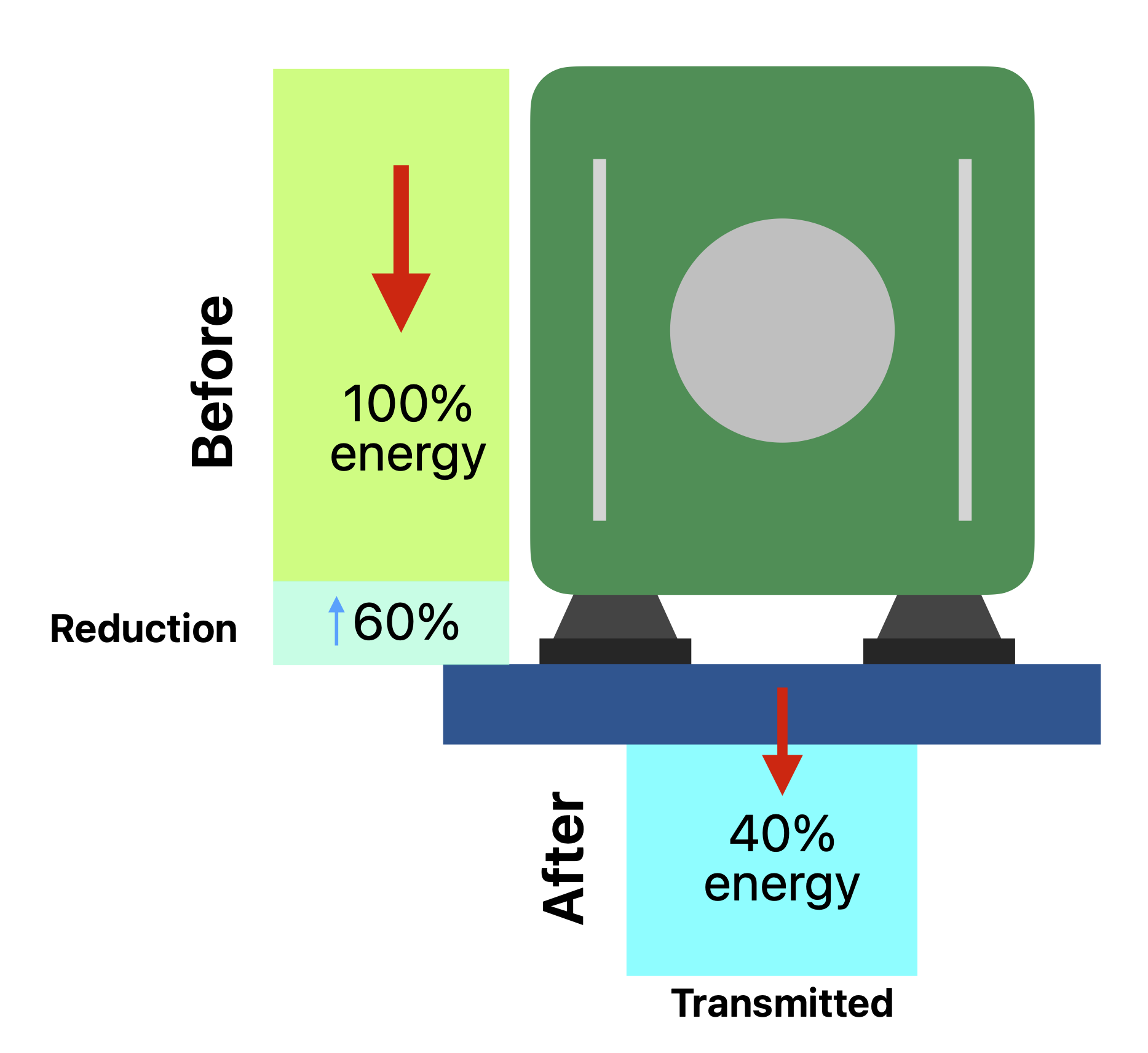
Figure 5.1.6 Illustration of isolation reduction.
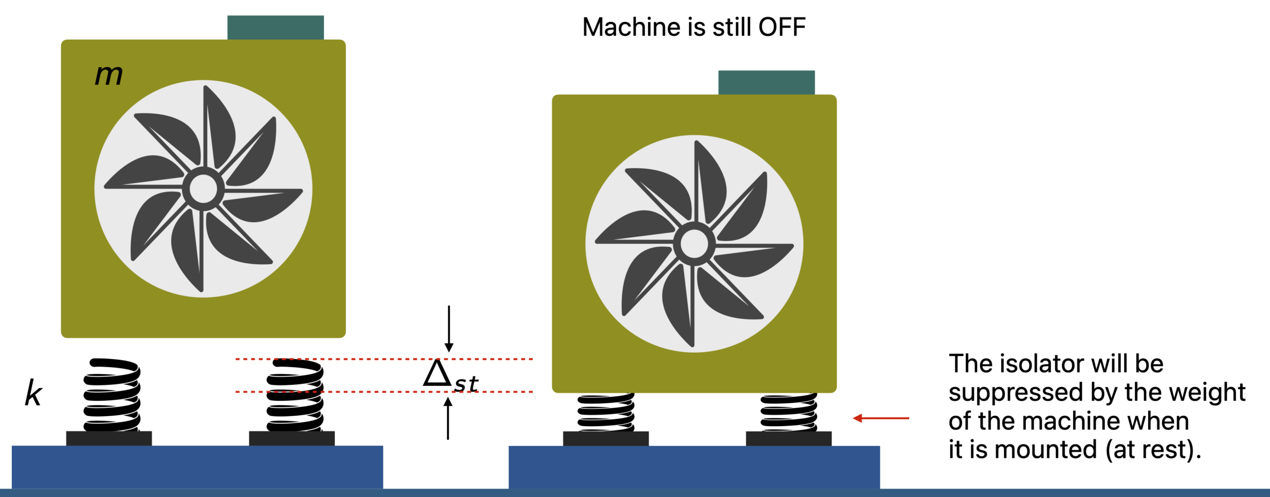
Static deflection
We have concluded that the transmissibility will be lower when the natural frequency,
is much lower, which means the smaller the stiffness (k) of the isolator, the better the isolation performance.
However, smaller stiffness means the “softer” the spring.
Can the ‘soft’ spring sustain the weight of the machine?
The deflection of the spring due to the machine’s weight is termed static deflection, and it is given by
\Delta_{st}=\displaystyle\frac{mg}{k}\phantom{xxxxxxxxxxxx}{\color{red}(5.1.17)}